Support Vector Regression machine learning with a radial basis function kernel

I recently completed a section in an amazing machine learning course I am taking on Support Vector Regression and thought I would share the dataset, the code and the visualization of the results below.

Dataset

Code

# Support Vector Regression (SVR)

# Importing the libraries
import numpy as np
import matplotlib.pyplot as plt
import pandas as pd

# Importing the dataset
dataset = pd.read_csv('Position_Salaries.csv')
X = dataset.iloc[:, 1:-1].values
y = dataset.iloc[:, -1].values
print(X)
print(y)
y = y.reshape(len(y),1)
print(y)

# Feature Scaling
from sklearn.preprocessing import StandardScaler
sc_X = StandardScaler()
sc_y = StandardScaler()
X = sc_X.fit_transform(X)
y = sc_y.fit_transform(y)
print(X)
print(y)

# Training the SVR model on the whole dataset
from sklearn.svm import SVR
regressor = SVR(kernel = 'rbf')
regressor.fit(X, y)

# Predicting a new result
sc_y.inverse_transform(regressor.predict(sc_X.transform([[6.5]])).reshape(-1,1))

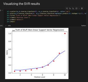
# Visualising the SVR results
plt.scatter(sc_X.inverse_transform(X), sc_y.inverse_transform(y), color = 'red')
plt.plot(sc_X.inverse_transform(X), sc_y.inverse_transform(regressor.predict(X).reshape(-1,1)), color = 'blue')
plt.title('Truth or Bluff (SVR)')
plt.xlabel('Position level')
plt.ylabel('Salary')
plt.show()

# Visualising the SVR results (for higher resolution and smoother curve)
X_grid = np.arange(min(sc_X.inverse_transform(X)), max(sc_X.inverse_transform(X)), 0.1)
X_grid = X_grid.reshape((len(X_grid), 1))
plt.scatter(sc_X.inverse_transform(X), sc_y.inverse_transform(y), color = 'red')
plt.plot(X_grid, sc_y.inverse_transform(regressor.predict(sc_X.transform(X_grid)).reshape(-1,1)), color = 'blue')
plt.title('Truth or Bluff (SVR)')
plt.xlabel('Position level')
plt.ylabel('Salary')
plt.show()

Visualization